Definition: Excel automation will streamline repetitive tasks such as updating data, formatting cells, sending emails, and even uploading files to SharePoint. Excel automation commonly uses custom-coded scripts written in VBA to complete tasks.
This article will guide you through everyday tasks that can be automated in Excel. A sample zip folder containing two workbooks with sample code will be provided. The samples will give you a hands-on opportunity to understand automation. While this article may not cover every automaton scenario, it will give you a base so you can get started building your tools!
Before diving in, understanding the distinction between Macros and VBA is essential. Macros are a collection of VBA code. The Excel Macro recorder records in VBA code. When you write your code in VBA, you create modules using the developer tab. These modules can then be called like any other Macro you see in the developer tab. If you want to learn how to record simple macros, here is a great video.
Here are some benefits of Excel automation:
- Increased efficiency – repetitive tasks can be completed with one button click.
- Error reduction – Since all steps are laid out logically in the code, there is no room for manual errors. Any errors in the code/logic can easily be updated.
- Better decision-making – Excel files will be easier to read, updated more often, and more accurate, leading to higher quality data.
Excel Automation Tips
- Sometimes advanced formulas are all that’s needed. For example SUMPRODUCT for row and column criteria instead of fumbling with a SUMIFS that seems to not work.
- Use helper columns – this will make troubleshooting each step in a calculation easier. Helper columns also come in handy for conditional formatting.
- If your workbook relies on many pivot tables, consider an alternative approach. Either better source data or native formulas to summarize source data. Too many pivot tables will increase the file size.
- Power Query is a great tool to import data, but VBA will give you more flexibility. Generally use PowerQuery for more simple projects/imports.
- Use Arrays – This means putting data into a variable type that is more memory efficient. When looping over large data ranges, put the range into an array, then manipulate the array as needed.
- Name your VBA modules accordingly so you know what code it contains.
- By default, VBA is case-sensitive. So when using IF statements, keep the case in mind. You can always convert things to lowercase using LCase to be sure the appropriate comparisons are made.
- When using native Excel functions inside of VBA, use Application. Instead of Application.WorksheetFunction. The application will not throw any run-time errors.
- You can use the underscore character to continue a VBA statement on a new line. This will make your code easier to read. In the sample workbook we provide, the email function uses this method.
- Use WITH to shorten your VBA code. This is commonly used only to type a range once, then use WITH to do multiple things with the range.
- When creating smaller macros, no need to declare all variables. This will save space and make your code easier to read. Declaring variables are only required when using arrays, dates, or when other function require a specific variable type. For larger macros, declaring variables might help give clarity to all the variable names being used and why (adding comments at top). Here is more information on declaring variables.
- Use the locals window in VBA to keep track and view the data inside variables. This is especially helpful for viewing arrays. You just need to add a breakpoint in your code. Highlight a line, then click F9. Then when the code runs, it will stop there, and all variables above that line will show in the locals window.
- You can set the visibility of sheets to “xlSheetVeryHidden”; that way, they not be shown with the native “Unhide.” You can then use a UserForm to prompt a password to show the tab. This is useful for payroll reports.
- Adding a progress bar is a nice touch for macros that take a long time to run, such as uploading many files to SharePoint.
The Sample Workbooks
Above is a link to the zipped folder with two workbooks. The “Automation Example Workbook.xlsm” contains common tasks that can be completed with VBA. Each tab has it’s own task. In addition to VBA, there is a tab with SUMPRODUCT formulas, string manipulation, and a conditional formatting example. We will explain each of the concepts in detail below.
The other file in the zip folder is “Source Data.xlsx”. This file has a list of sample sales rep salaries used as an import in the automation file.
The code to save copies of the workbook and import data assumes that the “Excel Automation” folder is on your desktop. Therefore, it is best to download the zip folder and unzip it on your desktop. If you decide to unzip it elsewhere, you must adjust the folder locations in the VBA.
Keep in mind this sample workbook doesn’t cover all scenarios you will encounter in your projects. But it will serve as a base to start automating tasks. In addition, mastering the concepts in this file will put you one step closer to being your company’s go-to Excel resource.
Advanced Formulas
Not all workbooks need VBA to be better automated. Many projects we encounter as consultants just need cleaner formulas.
SUMPRODUCT
SUMPRODUCT is great when criteria are in rows and columns, and you need to do counts or summaries. Because SUMPRUDCT takes arrays as arguments, the formulas are also ideal for summarizing data by fiscal year or other criteria. Below are two examples. The sample workbook has a lot of different examples you can study.
// Sum values by year, when the criteria column has dates
=SUMPRODUCT((YEAR(C20:C29)=year_value)*(D20:D29))

// Sum values by row and column criteria
=SUMPRODUCT((B35:B44="row_criteria")*(C33:F33="column_criteria")*(C35:F44))
INDEX + MATCH
INDEX + MATCH is excellent when you need to do a VLOOKUP, but the columns are out of order. For example, let’s say you need to return the employee region from the employee ID. If the employee region is in a column before the ID, then a VLOOKUP will not work. You could rearrange the columns, but the easiest solution is INDEX + MATCH. Below is how this formula would look.
// INDEX + MATCH
=INDEX(employee_data,MATCH(employee_id,employee_ids,0),column_to_return)
Unique Lists
Sometimes you don’t need VBA to create a unique list. For example, consider an accounting report that lists various account numbers and amounts. The report may list each transaction when you need a summary by amount. In this case, you can use a combination of the FILTER and UNIQUE function along with COUNTA.
Below is the formula found in the sample workbook. The FILTER function returns an array, and the unique function removes duplicates. When you wrap this inside the COUNTA function, blank rows are ignored.
// Get a unique list from a range
=IF(COUNTA(A64:A69)>0,UNIQUE(FILTER(A64:A69,A64:A69<>"")),"")
SUMIFS With Lookups
This formula can come in handy when you need to summarize amounts while also doing a lookup. For example, consider an account report that shows weekly metrics for various regions. The weeks can relate to periods. So might need to summarize all of Period 1 while referencing what weeks that period relates to.
Below is the formula that can be found in the sample workbook. It is the last formula on the “Advanced Formula” tab.
// SUMIFS with a lookup
=SUM(SUMIFS(C$74:C$79,$A$74:$A$79,IF($B$83:$B$86=TRIM(SUBSTITUTE($A89,"TOTAL","",1)),$A$83:$A$86),$B$74:$B$79,$B89))
String Manipulation
String manipulation is another key area to help streamline your Excel files. The most common example include:
- Determining if a string contains a word.
- Extracting a first name.
- Extracting an email.
- Getting a domain from a full website.
The sample Excel file has more examples, but here are a few formulas that can get you started.
// Does the cell contain a word
=IF(ISNUMBER(SEARCH("word",cell)),"Yes","No")

// Get the first name
=LEFT(cell,FIND(" ",cell)-1)

// Get an email from a string
TRIM(RIGHT(SUBSTITUTE(LEFT(cell,FIND(" ",cell&" ",FIND("@",cell))-1)," ",REPT(" ",LEN(cell))),LEN(cell)))
Custom Formulas
Messy workbooks can be better automated and simplified using custom formulas. Consider an example when calculating sales commissions. Certain regions might have a higher rate or a bonus commission for employees with a specific tenure. Instead of building a messy nested IF formula, you could create a custom one.
The custom formula would take a list of arguments you specify, just like any other formula. But the logic inside of the formula can be customized and easily updated when business logic changes. You can even further use VBA to pull in commission rates from another table. Below is an example of how a custom sales commission formula can be made.
Note: To create your own formula, click the developer tab, Visual Basic on the left, then insert a module and add the code below. The FUNCTION keyword will enable you to type the formula directly into the cell.
Function sales_commission(region As Variant, experience As Variant, sales As Variant)

'Set a variable that we can update based on conditions, setting to 0 here forces it to be a variant and not a string
base_commission_rate = 0
experience_bonus_rate = 0

If LCase(region) = "east" Then
base_commission_rate = 0.05

ElseIf LCase(region) = "west" Then
base_commission_rate = 0.06

End If

If experience > 5 Then
experience_bonus_rate = 0.03

End If

sales_commission = sales * (base_commission_rate + experience_bonus_rate)

End Function
Conditional Formatting
Adding highlights to cells or formatting a text based on conditions adds a layer to Excel automation. For example, conditional formatting is used to highlight duplicates, and errors or, most commonly, show accounting variances.
We recommend limiting your use of conditional formatting in VBA. It will be much easier to manage your conditional formatting with the help of helper columns and then custom-made formatting rules.
This conditional formatting example adds a helper column to a financial statement model. First, the helper column is labeled based on whether a higher variance is good or bad. And then, depending on the variance amount, the variance will be highlighted green or red. Because expenses can sometimes be shown as negative or positive, the helper columns make it easy to build two simple rules that cover all scenarios.
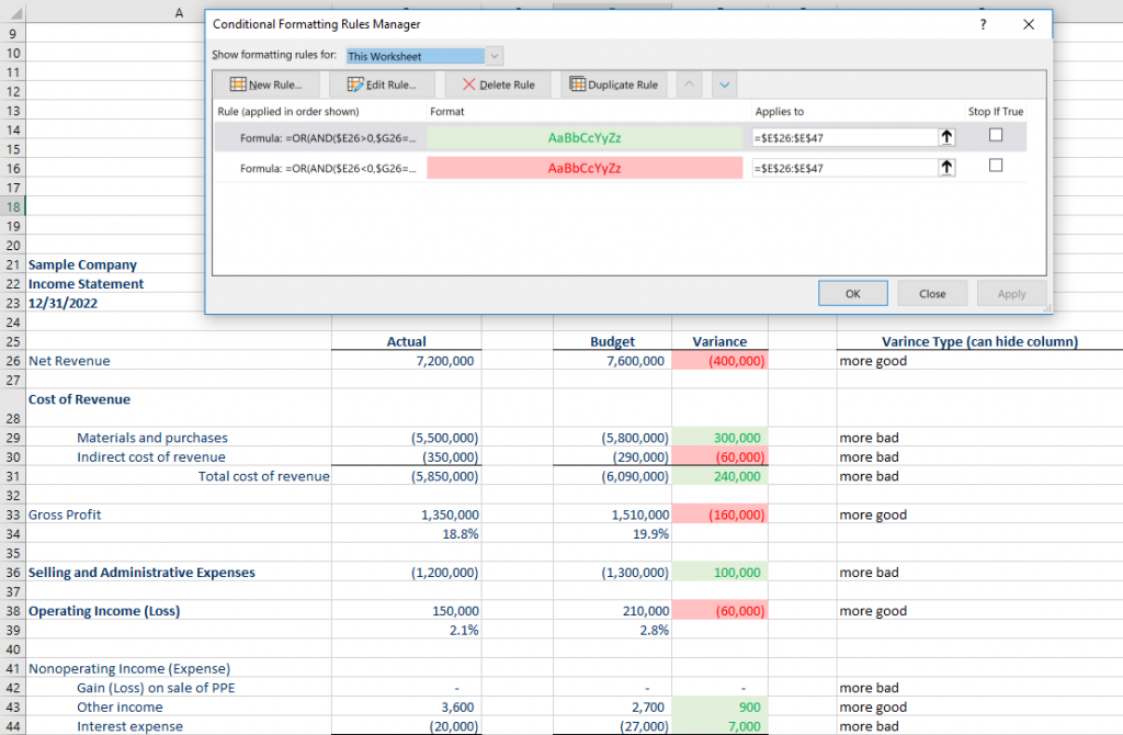
Remember: Custom-built conditional formatting rules follow the same logic as other formulas; you can lock cells and ranges and input a formula that would result in TRUE or FALSE. You can learn more about this here.
Looping Over Ranges
Looping over a range of cells is one of the core concepts of VBA and will help you automate many Excel tasks. When building dashboards, often, you can loop over the data to send emails to employees, upload a copy of the workbook to SharePoint, or mark a field as updated.
It’s easy to know where to start a loop for a range, but finding the last used cell can be tricky. For example, there could be a few blank rows, more data below those blank rows or some rows may have only partial data. Our preferred method is simply choosing a column and using End(XlUp).Row. Here is a great article detailing how you can find the last used cell.
Below is some sample code to loop over a range of cells. As the loop goes through each row, it grabs the sales rep’s name and places the rep’s name + a timestamp in a processed column.
Sub process_dashboard()

'Loop over the dashboard, put the date processed in column C

lastrow = ActiveSheet.Cells(Rows.Count, "A").End(xlUp).Row

For i = lastrow To 10 Step -1 'Start at bottom go to row 9
current_time = Format(Now, "mm/dd/yyyy hh:mm:ss")

With ActiveSheet
current_rep = .Cells(i, 1).Value
rep_region = Trim(.Cells(i, 2).Value)
End With

'Put a value in column C (column 3)
ActiveSheet.Cells(i, 3).Value = current_rep & " Processed on: " & current_time

'Now that you have the rep name and region, you can use data like that to save a copy of the workbook, edit the copied workbook, upload it to SharePoint, or send an email with the rep name
'Make sure all your code is before the next statement/span>

Next i

End Sub
Deleting Rows and Columns Based On Criteria
One of the most common tasks when automating a project would be to delete rows and columns based on criteria. A typical example would be saving each employee’s copy of a payroll workbook and ensuring that the source data has only their information.
There are two common ways to delete rows. Either loop through the rows and delete one row at a time if specific criteria are met, or use the Excel AutoFilter function to remove all rows at once. The AutoFilter method puts the data into a particular spot in memory and is ideal when you have large datasets that need to be edited quickly.
Here is an example of deleting rows using the logic of looping over a range.
Sub delete_rows()

'This method will find the last used row, start at the last row, and look for non-active values in column C
'The cell offset 2 is from column I
'Another way to do the last row lastrow = ActiveSheet.Cells.Find("*", SearchOrder:=xlByRows, SearchDirection:=xlPrevious)
lastrow = ActiveSheet.Cells(Rows.Count, "A").End(xlUp).Row

With ActiveSheet

For i = lastrow To 2 Step -1

If LCase(.Cells(i, 3)) = "non-active" Then
.Rows(i).Delete
End If

Next

End With

End Sub
Here is an example of deleting rows using the AutoFilter function. One of the significant benefits of using this method is that an array can be used as the search criteria.
Sub delete_rows_filter()

'Turn off the warning pop-up message
Application.DisplayAlerts = False

'This method will find the last used row, start at the last row, and look for non-active values in column C
'It is not possible to do "not equals to anything inside of an array". You would need to create an array full of items to filter instead
'To do not equal for a string use Criteria1:="<>non-active"
'1. Apply Filter - use a large range - or you could do a dynamic range and use the last row trick
  ActiveSheet.Range("cell:c5000").AutoFilter Field:=3, Criteria1:="non-active", Operator:=xlFilterValues 'need to update for correct ranges

'2. Delete rows
ActiveSheet.Range("a10:c5000").SpecialCells(xlCellTypeVisible).Delete

'3. Remove the filter
ActiveSheet.AutoFilterMode = False 'This is the best method

'To keep the filter you could use this instead
'ActiveSheet.ShowAllData - but if all data is deleted it would throw an error and you would then need to put "On Error Resume Next" in the line above

'This would keep the fitler but not throw any error if all data was removed - it would throw an error if the autofilter is not applied, so using this it might be a good idea to check for the autofilter first - if (ActiveSheet.AutoFilter.ShowAllData = true )
'ActiveSheet.AutoFilter.ShowAllData

'Turn on the warning pop-up message
Application.DisplayAlerts = True

End Sub
For simplicity, we will not include the code to delete columns here. But macro in the sample file finds the last used column and then loops over all used columns.
Importing Data
Importing data is also another cornerstone topic in Excel automation. When looking at online resources, many people may suggest using Power Query. While Power Query is a great tool and can remove columns and rows based on conditions, group rows, and automatically reimport data when the source changes, VBA methods will always provide you with more flexibility.
Consider an example where salary data needs to be imported before a payroll report is run. The excel dashboard might have a spot for “date last updated” in addition to a few check figures like employees not found. Using VBA to import the data will allow you to quickly populate the needed information in a dashboard and update the data.
Another typical example is that sometimes source data is too large to import. Instead of importing all the source data, you can import the data to an array, manipulate the data, then output the result to Excel. This month ensures that only the data you need is in the file, and no unnecessary information increases the file size.
The code below is in the sample workbook and can be used to import salary data from an external file. This code imports the data and does a few quality control checks. For example, it determines how many employees were in the source file, how many employees are missing from the source file, and places a diagnostic if an employee is not found in the source.
The key to this code is a custom-made function called “SheetToArray.” This function takes an Excel or CSV file and places the first sheet (or sheet name you specify) into an array that can easily be manipulated or searched. The “SheetToArray” function can be found in the “Mod99_General_Functions” module in the sample workbook.
Sub import_salary()

'Import the salary information from another file
'It assumes the source data is in the Excel Automation folder on your desktop, if you get any file location errors, change the path as needed

'Set employee array
Dim employee_id_array As Variant
Dim test_value As String 'The IsInArray function needs a string so define a string
Dim dToday As Date
dToday = Date
windows_userid = Environ$("UserName")
last_employee_row = ThisWorkbook.Sheets("Import Data").Range("A13").End(xlDown).Row
employee_id_array = Application.Transpose(ThisWorkbook.Sheets("Import Data").Range("B14:B" & last_employee_row).Value)

Dim source_data_array
source_data_array = SheetToArray("C:\Users\" & windows_userid & "\Desktop\Excel Automation\Source Data.xlsx")

total_csv_count = 0
not_found_in_ours = 0

'Loop over the first column of the CSV array and do some quality control checks

For outer = LBound(source_data_array, 1) To UBound(source_data_array, 1)

test_value = source_data_array(outer, 2)

'Search for the value in the array
found = IsInArray(test_value, employee_id_array)

If (test_value <> "") Then
total_csv_count = total_csv_count + 1
End If

If found = False Then
not_found_in_ours = not_found_in_ours + 1
End If

Next

ThisWorkbook.Sheets("Import Data").Range("B9").Value = total_csv_count
ThisWorkbook.Sheets("Import Data").Range("B10").Value = not_found_in_ours
ThisWorkbook.Sheets("Import Data").Range("B11").Value = dToday

'Now loop over the salary employee columns
For Each c In ThisWorkbook.Sheets("Import Data").Range("B14:B" & last_employee_row) 'use column B since it has the employee ID

employee_num = c.Value
c.Offset(0, 1).Value = simple_array_lookup(source_data_array, employee_num, 2, 3)  'Look in column 2, return column 3 from the source data

Next c

MsgBox "Salaries updated!"

End Sub
Some other import methods are connecting to a SQL database and getting data from a web API (like a POST or GET request). Both of these functions can be done with Power Query if you choose to do so. Again because automation relies mainly on VBA, using VBA for data imports will give you more flexibility. VBA also allows you to lay out the API request more flexibly and specify whether it is POST or GET. Here are some resources for more import methods.
Refreshing Pivot Tables
A simple but everyday automation task is updating pivot tables when the data changes. There are a few ways to do this in VBA. For example, you could either fresh all pivots at once, refresh all pivots on a sheet, or refresh a single pivot.
The code below puts a random number in the pivot table source data, then refreshes the pivot.
Sub refresh_pivot()

'This will edit one of the source data cells, then refresh the pivot

random_number = (Int(6 * Rnd) + 1) * 10000
ThisWorkbook.Sheets("Pivot Data").Range("D4").Value = random_number

ThisWorkbook.Sheets("Pivot Table").PivotTables("PivotTable1").PivotCache.Refresh

'Or you could refresh all tables at once
'ThisWorkbook.RefreshAll
Exit Sub 'The code below won't run - but we can demonstrate an example
'This logic can be used to loop over sheets then pivot tables
Dim piv As PivotTable
For Each piv In Sheet6.PivotTables 'Instead of sheet 6 put your sheet name
piv.PivotFields("Date").ClearAllFilters
piv.PivotFields("Date").CurrentPage = Range("Date")
Next piv

End Sub
Cleaning and Organizing Data
Automation often involves the need to clean or organize data. This could include eliminating duplicates, removing unnecessary data, or correctly formatting (such as GL data missing the whole account numbers). As mentioned early, Power Query can handle some of these tasks, but using VBA will give more options when cleaning data.
Consider an example of an Excel report that pulls data from Oracle Smart View. There could be a requirement to put a specific subset of data on a supporting schedule. The key to this is using arrays. Once the source data is an array, it is simple to manipulate and place it on a new tab or range.
The code below takes a range, places it into an array, searches for east region sales reps, places those into a new array, and finally outputs the new array to cell F10 on the same sheet. Keep in mind that as the data is being looped over, you could remove unnecessary items or build advanced criteria on multiple columns in the array.
Array Notes: This code uses UBound to resize a cell selection. This means taking a one-cell Excel range and resizing it to the number of rows and columns the multidimensional array contains.
Sub clean_data()

'This macro will put all the sales reps into an array.
'The array is looped through to grab the east region reps and they are put into another array.
'We then place that other array into cell F2. This logic is useful to clean or organize source data.
'You can view the arrays by going up to view->locals window

Dim source_array As Variant
Dim clean_array(5000, 1) 'Array elements start at 0 - 5001 rows to make it big enough, 2 columns (starting at 0 so 0,1)
'You could do clean_array(1 to 5000, 1 to 2) to start and at specific values instead of 0
'You can only redim (resize) the second part/last value of an array.
'So you can set the first value to be large enough or set it from another value. You could use a transpose trick, which is found here:
'https://stackoverflow.com/questions/67444220/excel-vba-how-do-you-add-a-row-to-a-2d-variant-array-while-preserving-old-arra

source_array = Range("a10:d20").Value 'You can use a dynamic range if you want

'Loop through the entire array
Dim i As Long, j As Long
row_counter = 0
For i = LBound(source_array, 1) To UBound(source_array, 1) 'Loop over the rows in the array

If source_array(i, 2) = "East" Then
clean_array(row_counter, 0) = source_array(i, 1)
clean_array(row_counter, 1) = source_array(i, 3)
row_counter = row_counter + 1 'Only east regions will be incremented and thus the array will only has east regions in order with no blank gaps
End If

For j = LBound(source_array, 2) To UBound(source_array, 2) 'Loop over the columns in the array - you don't need to do this, but we included it here so you can experiment

Next j

Next i

'Now place the new array in cell F9
'This version below will put the full 5000 rows in. But since we have the row_counter, we can use that instead
'ThisWorkbook.Sheets("Clean Data").Range("F10").Resize(UBound(clean_array, 1) + 1, UBound(clean_array, 2) + 1).Value = (clean_array) '+1 means adjust for starting at 0, so add an extra value to the range resize

ThisWorkbook.Sheets("Clean Data").Range("F10").Resize(row_counter, UBound(clean_array, 2) + 1).Value = (clean_array) '+1 means adjust for starting at 0, so add an extra value to the range resize

End Sub
Saving Copies of a Workbook
For projects like payroll, you might need to save a workbook copy for each employee. To automate this process (if not opting for a free online payroll system), you can build a dashboard, loop over the employees, and then save a copy of the workbook for each row. When a copy of the workbook is saved, you can then manipulate it to remove data not belonging to the employee or add notes and custom calculations.
When you save a copy of the workbook, there is one key thing to take note of. The function to save a copy (SaveCopyAs) must keep the file extension the same. Since the Macro is likely in an XLSM extension, the new file must also be in XLSM. There are some workarounds, but it will get messy when processing multiple books. We recommend just keeping the XLSM extension, and it needs just a password to protect the VBA project (so people can’t edit).
The code below will loop over a dashboard and save a copy if column C is “Yes.” The code will then manipulate the new workbook deleting unneeded sheets and adding a new sheet.
Sub save_copy()

Application.DisplayAlerts = False 'Switching off the alert button
Application.ScreenUpdating = False


'Loop over the dashboard, put a process date in column C
windows_userid = Environ$("UserName")
last_employee_row = ThisWorkbook.Sheets("Save Copy of Workbook").Range("A10").End(xlDown).Row
employee_id_array = Application.Transpose(ThisWorkbook.Sheets("Save Copy of Workbook").Range("B10:B" & last_employee_row).Value)

Dim source_data_array

lastrow = ActiveSheet.Cells(Rows.Count, "A").End(xlUp).Row

For i = lastrow To 9 Step -1 'Start at bottom go to row 9
current_time = Format(Now, "mm/dd/yyyy hh:mm:ss")

With ActiveSheet
current_rep = .Cells(i, 1).Value 'Column 1
rep_region = Trim(.Cells(i, 2).Value) 'Column 2
process_book = Trim(.Cells(i, 3).Value) 'Column 3
End With

If process_book <> "Yes" Then
GoTo next_rep
End If

'Now create a dynamic file name
'If uploading to SharePoint, just change the folder name to the synced folder location
file_name = ("C:\Users\" & windows_userid & "\Desktop\Excel Automation\" & current_rep & ".xlsm")
ThisWorkbook.SaveCopyAs Filename:=file_name 'Savecopyas you need to keep the extension the same. So in this case the file will be xlsm
Dim copiedWorkbook As Workbook
Set copiedWorkbook = Workbooks.Open(file_name)  'Now you can manipulate the new book as needed

'Loop over the sheets in the copied book, only keep the Save Copy of Workbook tab

Dim ws As Worksheet

For Each ws In copiedWorkbook.Worksheets
If ws.Name <> "Save Copy of Workbook" Then
ws.Delete
End If
Next ws

'Insert a sheet
Set ws = copiedWorkbook.Sheets.Add(After:= _
copiedWorkbook.Sheets(copiedWorkbook.Sheets.Count))
ws.Name = "New Sheet"
copiedWorkbook.Sheets("New Sheet").Range("A1").Value = "This is the new sheet"

copiedWorkbook.Save
copiedWorkbook.Close SaveChanges:=False

current_time = Format(Now, "mm/dd/yyyy hh:mm:ss")
ActiveSheet.Cells(i, 4).Value = current_time

next_rep:
Next i 'Next sales rep

Application.DisplayAlerts = True 'Switching on the alert button
Application.ScreenUpdating = True

MsgBox "Workbooks processed!"

End Sub
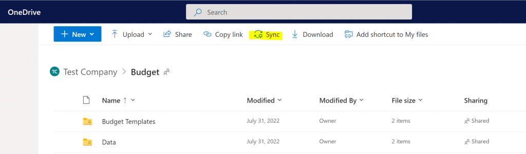
Uploading to SharePoint
To upload a file to SharePoint, you first want to sync the SharePoint folder to your local machine. The syncing process creates a folder on your C drive that you can reference when saving files. For example, the sample below would sync the “Budget” folder to the C drive along with subfolders.
Previously, an alternative method involved manually mapping a SharePoint folder to a network drive. However, this had many flaws, including needing to set permissions in internet explorer. For reference, here is an article demonstrating this.
Sending Emails
When a report is processed, you will send an email letting the parties know the process is complete. In addition, you can send an email from Excel to save a step and further streamline your project!
There are two methods to send emails. CDO or by just creating an Outlook object.
The Outlook object method is the most common. You create an Outlook object in VBA and then add some additional settings to the object, like attachments. You can even add an option to keep the email open or send it immediately. Keeping the email open is preferred; that way to can make modifications before sending.
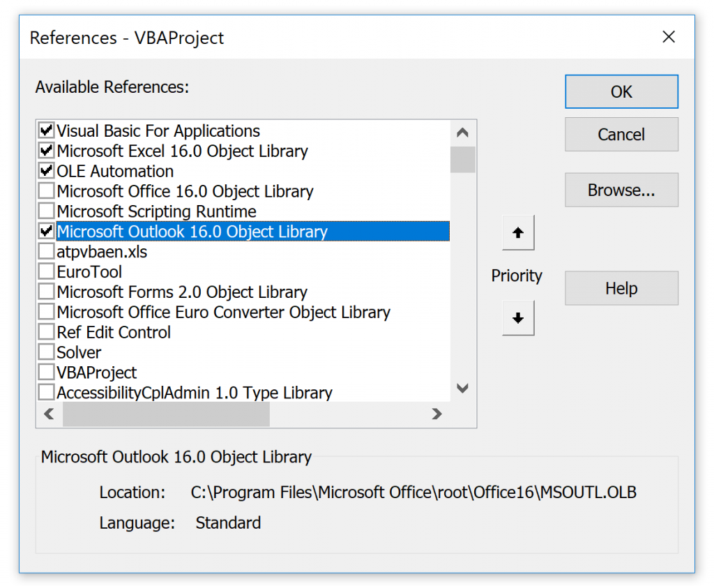
To use the Outlook object method, you need to ensure the “Microsoft Outlook 16.0 Object Library” is checked in Tools > References.
The code below uses a custom email function to send the email. That custom function can be found in the “Mod98_Email_Functions” module of the sample file. The function takes only one required argument, the send to email, then some optional arguments such as attachments and the email body.
Sub send_emails()

'The email function needs a string, so a string is declared header_remove()
Dim rep_email As String

lastrow = ActiveSheet.Cells(Rows.Count, "A").End(xlUp).Row

For i = lastrow To 10 Step -1 'Loop over the dashboard. Start at the bottom go to row 10

With ActiveSheet
current_rep = .Cells(i, 1).Value
rep_email = Trim(.Cells(i, 2).Value)
process_email = Trim(.Cells(i, 3).Value)
End With

If process_email = "Yes" Then

Call send_email( _
 _
send_to:=rep_email, _
from:="sender@example", _
cc:="sender@example.com", _
subject:="This is the subject", _
body:="<p>Hello,</p><p>This is an HTML email! You can easily add <a href = 'www.google.com'>links</a> to the message. Links are often used to email SharePoint files.</p>", _
attachment:="", _
auto_send:="no" _
)

End If

Next i

End Sub
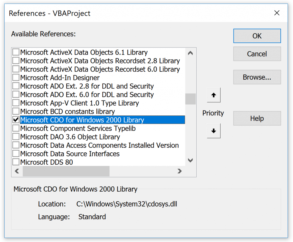
If Outlook is not installed on your machine or security restrictions prevent you from sending a VBA email with an Outlook object, you can use the CDO method. This method would require some help from IT to get the server name, port, and account name. You also need to ensure the “Microsoft CDO for Windows 2000 Library” is checked under Tools > References.
Saving as a PDF
Some projects may require saving a particular tab or the entire workbook to a PDF. The sample code for this is pretty straightforward. This reference goes over some additional scenarios and options for saving to a PDF.
Sub save_pdf()

'Save of copy of the current sheet as a PDF

windows_userid = Environ$("UserName")

Dim saveLocation As String
saveLocation = "C:\Users\" & windows_userid & "\Desktop\Excel Automation\Sample PDF.pdf"

'Save Active Sheet(s) as PDF
ActiveSheet.ExportAsFixedFormat Type:=xlTypePDF, _
Filename:=saveLocation

End Sub
Consulting Services
For consulting projects, we simply charge $50 an hour. You can schedule an Excel Consultation with us to review your project and get a quote.
One of the benefits of working with an established tech company is access to professionals that solve any problem within your project scope. For example, some projects may require better source data. In those cases, we can help write SQL queries or views. Sometimes Excel is not the best option; in that case, we can help build a custom application or recommend different tools.

Ready To Start?
Create your own survey now. Get started for free and collect actionable data.