Updated 1/11/2026
Standard Deviation Calculator (With Variance)
Standard deviation and variance measure how much a dataset deviates from the mean. Variance is defined as the average of the squared differences from the mean and is used to compute standard deviation. Standard deviation is the square root of the variance.
This calculator computes standard deviation, variance, mean, sum, and margin of error. Paste your data to calculate results instantly. A low standard deviation or variance indicates values clustered near the mean, while higher values indicate greater spread.
How to Calculate Standard Deviation
Below is an example of 6 test scores from a class to walk through an example calculation:
Test scores:
78, 88, 81, 92, 65, 58
The above example can be condensed to the following formulas:
Population Standard Deviation
(All elements from a data set - e.g 20 out of 20 students in class)
The population standard deviation is used when the entire population can be accounted for. It is calculated by taking the square root of the variance of the data set. The following equation can be used in this scenario:
Where,
σ = Population standard deviation
∑ = Sum of..
xi = An individual value..
μ = Population mean
n = Number of values in the population data set
Sample Standard Deviation
(One or more elements from a data set - but not 100% of elements - e.g 100 out of 300 students taking a computer class)
Sometimes it is not possible to capture all the data from a population, so we use a sample. The sample standard deviation formula uses the sample size as "n" and then makes an adjustment to "n". This adjustment, ("n-1" below) is referred to as degrees of freedom. The version below is used in most entry level statistical courses. While it is a better estimate compared to just using the population started deviation, this version still has significant bias for small sample sizes (less than 10).
Where,
s = Sample standard deviation
∑ = Sum of..
xi = An individual value..
x̄ = Sample mean
n = Number of values in the sample data set
How to Interpret Standard Deviation
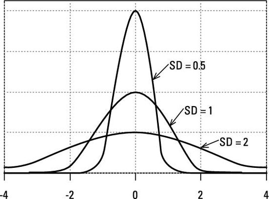
Standard deviation quantifies the amount of variation or dispersion of a data set. The standard deviation shows how widely the data set distributed about the mean. A smaller standard deviation indicates that more of the data is clustered about the mean. A larger one indicates the data set is more spread out.
Generally speaking, data is normally distributed. This is important as it then can be inferred that normally distributed data follows a bell shaped curve. That bell shaped curve can give us further insights.
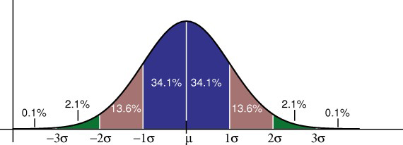
The above graph shows the rules for normally distributed data. 68.2% of responses are within 1 deviation of the mean, 95.4% of responses are within 2 deviations of the mean, while 99.6% of the data is within 3 deviations of the mean.
Example: If a question in your survey asks for annual income, the mean could be $35,000 with a standard deviation of $5,000. From the empirical rule, we could assume that 68% of total responses fall somewhere between $30,000 and $40,000. We could also assume 95% of the data falls between $25,000 and $45,000.
This data would help ensure a successful marketing campaign. You would now be able to create a campaign specific to your largest demographic!
How to Interpret Variance
Variance also measures the amount of variation or dispersion of a set of data values from the mean.
As mentioned, variance takes the average of all the squared differences from the mean. Standard deviation takes the square root of that number. Thus, the only difference between variance and standard deviation is the units. For example, if we took the times of 50 people running a 100-meter race, we would capture their time in seconds. When we compute the variance, we come up with units in seconds squared. Seconds squared aren't useful, so to get back to regular second units, we take the square root of the variance.
The variance takes the squares of the difference compared to the mean (as opposed to the absolute value) for two important reasons: squaring always gives a positive value and squaring emphasizes larger differences.
Standard Error of the Mean
If you look at a sample of data that is normally distributed, the mean should be close to the population mean. But depending on the sample you took, the data might be spread out compared to the mean, and thus your sample mean might differ compared to the population mean. As in the above example, if we took the times of 50 people running a 100-meter race, we might notice the mean is 16 seconds. If you took a sample of 100 people, the mean might be 15 seconds flat. The population mean would be closer to 15 seconds, as opposed to 16 seconds.
The larger the sample, the closer your data set will be grouped near the mean.
The larger the sample, the better conclusions you can draw. In the real world it might not be possible to sample the entire population for a set of data. In that case we would need to compute an error to determine how close our sample mean is compared to the population mean. This is called the standard error of the mean, also referred to as standard error. A low standard error indicates your sample mean is close to the population mean. A high standard error indicates your sample mean is father away from the population mean.
The equation for computing the standard error is as follows:
Where,
SE x̄ = Standard Error
σ = Population Standard Deviation
n = Number of values or observations in the sample data set
Using the standard error, a confidence interval can be computed for the range for the true mean. The equation to find out the confidence interval for the mean would be:
Where,
x̄ = Sample mean
Z = Z-Score for your confidence level (see table below)
SE x̄ = Standard error
| Desired Confidence Interval | Z-score |
| 80% | 1.28 |
| 85% | 1.44 |
| 90% | 1.65 |
| 95% | 1.96 |
| 99% | 2.58 |
Standard Deviation Use Cases
Standard deviation and variance are used anywhere teams need to understand consistency, spread, and variability across numeric data. Below are common applications across research, analytics, and performance measurement.
Research Design
Standard deviation helps researchers evaluate how consistently respondents answer a question, not just what the average response is. High variability often signals disagreement or polarized opinions, while low variability indicates alignment.
These measures are frequently used when analyzing research questions, especially in rating-scale and opinion-based surveys, where understanding the response distribution is critical.
Training Evaluations
In training and development, standard deviation helps determine whether results are consistent across sessions, trainers, or time periods. A strong average score with high variance may indicate uneven delivery or mixed outcomes.
This approach is commonly applied when analyzing results from a training evaluation form to compare performance over time or across teams.
Financial Modeling
Variance and standard deviation are core inputs in many business and financial models. They are used to quantify uncertainty, risk, and volatility in projections and performance metrics.
These calculations are commonly applied in budgeting, forecasting, and scenario analysis within financial modeling services, where understanding variability matters as much as the average outcome.
Demographic Analysis
When working with continuous data such as income, age, or spending, standard deviation helps explain how the spread differs across demographic or regional groups.
This is especially useful when analyzing survey results collected using a demographics survey template, where understanding variability across segments provides more profound insight than averages alone.